Hodgkin and Huxley's giant squid axon model

I deeply regret that I must begin this post by informing you that the entity in question is a giant axon from a squid, and not an axon from a giant squid. I can only imagine your disappointment on learning this fact - I recall that mine was considerable.

The models of heart cells that I'm working on at the moment are all based off a mathematical model from way back in 1952, created by Alan Hodgkin and Andrew Huxley. They described the electrical signal that passes down the axon of a squid's nerve cell when it is excited. The axon that controls the water jet propulsion system of a squid is particularly large, and easy to use in experiments.

The basis of this mathematical model is an understanding of the cellular features as components in an electrical circuit.* Just like in heart cells, the electrical signal is caused by the movement of charged particles, called ions, across the cell's outer membrane. The membrane of a neural cell acts like a capacitor, which means that ions accumulate on one side of the membrane, allowing it to store charge. This makes one side of the membrane more positive than the other side, leading to a voltage across the membrane.

This graph shows how the voltage across the membrane changes when the cell is stimulated.

An electrical impulse in an axon

The flow of ions across the membrane acts as an electrical current. Three types of ionic current are considered in this model: the sodium () ions that flow into the cell and cause depolarisation of the membrane, the potassium () ions that flow out to repolarise the membrane, and the "leak" current (a mixture of ions, including chloride ions), which flows in both directions.

Circuit description of nerve cell

The electrochemical gradients that power the flow of each type of ion are modelled as batteries, and the ion channels that permit ions to pass are represented by variable resistors.

is the stimulus current that the cell receives from outside.
and are the sodium, potassium and leak currents, respectively.
is the capacitance of the membrane (i.e. its ability to store charge)
is the membrane voltage
and are the resistance of the membrane to letting each type of ion through
and are the membrane potentials at which the flow of sodium, potassium or leak ions (respectively) through the membrane is zero.

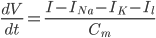
Since the current across the capacitor depends on the change in voltage over time and on the capacitance (
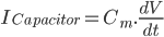
), and the four components of the current (that are wired in parallel) all add up to the stimulus current (), a unifying differential equation can be created.

Where , i.e. the difference between the current membrane voltage and the usual, or "resting" voltage.

The next part of the paper deals with the gating mechanisms for the ion flows. My plan is to tackle that next week!

The original paper is available free from PubMed Central here. There's also a very good description of its content on Wikipedia, and an illustrated XML version of the model at the CellML model repository.

I put together some MATLAB code to solve the equations described in the paper - you can download and view or run the source code here.

One of the most interesting features of this paper are its descriptions of a possible mechanistic basis for the permeability of the cell membrane to ions. This paper was written long before ion channels were discovered and characterised in mammalian cells, so it's amazing how accurately it describes the action of the nerve cell. (A very readable account of the history of ion channels is available on Montana State University's webpage here, incidentally).

* which I'm sure is a helpful explanatory device for people who have the foggiest concept of how electricity works. I am not one of these people. I've relied on some A-level revision websites and my various physicist chums/siblings for that.

...

Modifying a FLAME model

As I mentioned in my previous post about my adventures in FLAME modelling, I started out with code from my lecturer. I started with three two-dimensional models, each of which contained a different type (genus) of bacteria (Vibrio, Sar11 and "Bacteria X"). Each bacteria agent had X and Y co-ordinates, an ID and a radius. The radius was different for each type of bacteria, and it defined the rules that applied to that bacteria. They moved around by Brownian motion, and if they hit a virus there was a certain probability that they would be killed. The phages moved around in a similar fashion.

My code can be downloaded from here. In this post, I'm going to take you through how I converted these three models into a single model, added a third dimension, and persuaded the viruses and bacteria to replicate. This is a tale of how it's possible to do some quite cool things to a program even if you don't fully understand how it works.

If you're particularly interested, you can download a PDF of the report I handed in here. It starts with a brief review of a mathematical bacteriophage model, then goes on to the FLAME model in the second half (page 2). I got a mark of 95% for it, so I'm showing it off to everyone ^_^

Continue reading Modifying a FLAME model

...

Running FLAME models at the Linux command line

Update: I've written another post about how I edited the model.

Last week, I modified a FLAME model to make it 3D and added some other features (with help from my John). This animation is of the model running, with me wiggling it around a bit to show the 3D-ness, and then leaving it be. There are explosions!

3D FLAME model of bacteria-phage interactions

I think it's pretty cool. It represents a community of bacteria being attacked by viruses. These viruses - known as "bacteriophages" - could be really useful for treating infections, because they can kill bacteria which are resistant to traditional antibiotics.

In order to work out what dosage to use, and when to apply it, we need to know more about how bacteria and viruses interact with each other. This is difficult to study in real life, since viruses are so tiny - but by using computer models, we can make better approximations of how they behave.

The animation shows three types of bacteria, represented by green, blue and pink spheres. The orange dots are viruses. When a bacterium is infected by one of the viruses, it bursts, releasing lots of new viruses. Each virus and bacterium is an "agent" inside the model, and they each follow a particular set of rules, and carry pieces of information. I was using a piece of software called "FLAME" for this.

FLAME uses C and XML to make rules for the agents in a model. I found the documentation a bit obtuse, so I thought I'd make a blog post about exactly what I did, in case it was useful to anyone.

Initially, you need to install a set of programs - gcc, xparser, libmboard, and the FLAME visualiser. The installation instructions on the website are quite straight-forward, so I'll start my tutorial by talking about running a model.

Running a model in FLAME using the Linux command line

You can download my model code from here. It contains 4 files.

  • 0.xml describes the starting state of all the agents in the model
  • phageAndBacteriaV6.c contains all of the functions that the agents use
  • phageAndBacteriaV6.xml describes all the agents, and the messages they send each other
  • visual-rules.xml dictates how the model will be visualised

You start by using the xparser program on the xml file. I saved all my files in /home/beth/models/ so that is the location that I will use in my command line work - you should substitute it for your working folder. So: open up a terminal. Next, navigate to the directory where you have installed xparser and run

./xparser /home/beth/models/phageAndBacteriaV6.xml

This will create a load of files in home/beth/models. Navigate to /home/beth/models and run

make

This creates the model programs, most importantly one called main. You can then run the model, giving the number of iterations you want (in this case, 100) and the location of the 0.xml file (in this case, ./0.xml)

./main 100 ./0.xml

This creates a load of xml files, numbered 1 to 100. Each one contains information about every single agent in the model at a particular time step. Now, these don't look very exciting in themselves, but this is where the flame visualiser comes in.

Navigate to where you've installed the visualiser and run

./flame_visualiser

A window should pop up. Go to "File" > "Open" and find visual-rules.xml. If you click on "Open Visual Window", you should now see lots of lovely spheres. It's a fairly straight-forward program to use - you can drag the picture around, start and stop the animation, go back and forward through the iterations, and zoom. If you have a tiny screen, you can grab and move the window by holding down Alt when you click & drag.

I made my animation by opening "Image Settings" and then setting the iteration to 0 and clicking "Start Animation." This saves a series of numbered images. You can rotate the picture while you're recording if you fancy. Then I opened up The GIMP, clicked "File" > "Open As Layers" and selected all 100 images. Then I saved the image as a .gif, selecting "Save As Animation".

So that's how to run an existing model, and make a pretty picture. In my next post, I talk about how to edit one.

Edit: I forgot to add, the visual-rules.xml document was generated by the flame visualiser. You need to give each type of bacteria a radius and a colour using the visualiser, and an xml document will be generated.

...